remotes::install_github("hfshr/bitmexr")bitmexr: An R client for BitMEX cryptocurrency exchange.
Bitcoin
R
How bitmexr came to be.
While writing my previous post, I was surprised to find that there was no R related package for the cryptocurrency exchange BitMEX. While cryptocurrency itself is a somewhat niche area, BitMEX is one of the largest and most popular exchanges, so I had assumed someone would have already put together something in R for accessing data through BitMEX’s API. As I could find no such package, I drew inspiration from the few ‘crypto’ related packages that do exist, and set about creating a package that would provide a R users with a set of tools to obtain historic trade data from the exchange..
BitMEX has a very detailed API that allows users to perform essentially every action possible on the site through the API. This ranges from simple queries about historic price data through to executing trades on the platform. Initially, I just wanted the package to be able to easily access historic data for research purposes, however it would be relatively straightforward to implement additional features such as executing trades through the API.
And like that, bitmexr was born…
Currently you can install bitmexr from github, but hopefully the package will be on CRAN soon.
bitmexr
bitmexr is a relatively simple package that enables the user to obtain data about trades that have been executed on the exchange. The API supports trade data to be returned in two forms:
Individual trade data
- Details about individual trades that have taken place on the exchange
Bucketed trade data
- A summarised form of individual trade data where individual trades have been “bucketed” into one of the following time intervals; 1-minute, 5-minute, 1-hour or 1-day.
To access this data, bitmexr has two core functions:
trades()for individual trade data
library(bitmexr)
library(dplyr)
library(rmarkdown)
library(knitr)
library(tidyquant)
library(purrr)
library(gganimate)


trades(symbol = "XBTUSD", count = 5) %>%
  select(-trdMatchID) %>% # unique trade identifier, not particularly interesting
kable()| timestamp | symbol | side | size | price | tickDirection | grossValue | homeNotional | foreignNotional |
|---|---|---|---|---|---|---|---|---|
| 2022-03-13 20:18:49 | XBTUSD | Sell | 400 | 38710.0 | ZeroMinusTick | 1033324 | 0.0103332 | 400 |
| 2022-03-13 20:18:49 | XBTUSD | Sell | 200 | 38710.0 | ZeroMinusTick | 516662 | 0.0051666 | 200 |
| 2022-03-13 20:18:49 | XBTUSD | Sell | 100 | 38710.0 | MinusTick | 258331 | 0.0025833 | 100 |
| 2022-03-13 20:18:49 | XBTUSD | Sell | 100 | 38713.5 | MinusTick | 258308 | 0.0025831 | 100 |
| 2022-03-13 20:18:49 | XBTUSD | Sell | 100 | 38715.5 | MinusTick | 258294 | 0.0025829 | 100 |
bucket_trades()for bucketed trade data
bucket_trades(symbol = "XBTUSD", count = 5, binSize = "1d") %>%
kable()| timestamp | symbol | open | high | low | close | trades | volume | vwap | lastSize | turnover | homeNotional | foreignNotional |
|---|---|---|---|---|---|---|---|---|---|---|---|---|
| 2022-03-13 | XBTUSD | 38714.5 | 39480.0 | 38645.5 | 38794.0 | 63987 | 377767900 | 39060.82 | 1400 | 9.671287e+11 | 9671.287 | 377767900 |
| 2022-03-12 | XBTUSD | 39418.0 | 40245.5 | 38239.0 | 38714.5 | 141479 | 979194400 | 39062.35 | 1700 | 2.506753e+12 | 25067.534 | 979194400 |
| 2022-03-11 | XBTUSD | 41954.5 | 42037.0 | 38420.0 | 39418.0 | 181394 | 1351599500 | 39651.86 | 6500 | 3.408674e+12 | 34086.744 | 1351599500 |
| 2022-03-10 | XBTUSD | 38723.5 | 42596.5 | 38641.5 | 41954.5 | 167006 | 1079137900 | 41338.54 | 200 | 2.610491e+12 | 26104.907 | 1079137900 |
| 2022-03-09 | XBTUSD | 37967.0 | 39381.0 | 37857.0 | 38723.5 | 156917 | 1087892900 | 38651.68 | 3700 | 2.814608e+12 | 28146.078 | 1087892900 |
These functions allow the user to quickly return historic trade/price data that have been executed on the exchange.
map_* variants
In addition to the core functions, the packages contains map_* variants of each function. These functions were implemented to address two restrictions within the API:
- The maximum number of rows per API call is limited to 1000
- The API is limited to 30 requests within a 60 second period
The map_* functions are useful for when the data you wanted to return is greater than the 1000 row limit, but you want to avoid running in to the request limit (too many request timeouts may lead to an IP for up to one week).
For example, say you want to get hourly bucketed trade data from the 2019-01-01 to 2020-01-01.
bucket_trades(startTime = "2019-01-01",
              endTime = "2020-01-01",
              binSize = "1h",
              symbol = "XBTUSD") %>%
  filter(timestamp == max(timestamp)) %>%
  select(timestamp) %>%
kable()| timestamp |
|---|
| 2019-02-11 15:00:00 |
The first 1000 rows have only returned data up until 2019-02-11. To obtain the rest of the data, you would need to pass in this start date and run the function again, repeating this process until you had the desired time span of data.
This is where the map_* variants come in handy.
map_bucket_trades(start_date = "2019-01-01",
                  end_date = "2020-01-01",
                  binSize = "1h",
                  symbol = "XBTUSD",
                  verbose = FALSE) %>%
  paged_table()
If verbose is set to TRUE information about what is going on and a progress bar showing how long is left is printed to the console. Now the end date is what we wanted.
map_trades() works in a similar way, however because the number of each trades for a specified time interval is not known in advance, no progress bar is printed. Instead, the last date of the most recent API call is printed to provide an indication of how long is left (relative to the inputted start and end date). This function uses a repeat loop that will keep calling the API until the start date is greater than the end date.
The following example gets the every trade for “XBTUSD” between 12:00 and 12:15 on the 6th June 2019.
map_trades(symbol = "XBTUSD",
           start_date = "2019-06-01 12:00:00",
           end_date = "2019-06-01 12:15:00") %>%
  select(-trdMatchID) %>% # unique trade identifier, not particularly interesting
  paged_table()
This short 15 minute time interval resulted in ~6000 trades being returned - consequently this function should only be used for very specific time intervals where you require individual trade data. A warning is given if a time interval of greater than 1 day is provided. For example:
include_graphics("images/warning.png")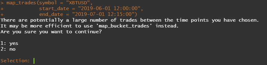
In contrast, using bucket_trades() with the smallest binSize setting summarises those 6000 rows into 16 - one for each minute between 12:00 and 12:15.
bucket_trades(symbol = "XBTUSD",
              startTime = "2019-06-01 12:00:00",
              endTime = "2019-06-01 12:15:00",
              binSize = "1m") %>%
  paged_table()
Use with other packages
bitmexr simply allows the user to get the data. With data in hand, there are several fantastic packages that can be used to help explore, visualise the data further. Two personal favourites are tidyquant(Dancho and Vaughan 2020) and gganimate(Pedersen and Robinson 2020).
Combining bitmexr and tidyquant makes it easy to perform financial analysis. For example, comparing the monthly returns of the two most traded contracts on Bitmex
btc_year <- map_dfr(c("XBTUSD", "ETHUSD"), ~map_bucket_trades(symbol = .x,
                                                              binSize = "1d"))
Earliest start date for given symbol is: 2018-08-02 09:06:10.
Continuing with earliest start datebtc_year %>%
filter(timestamp > "2018-08-01") %>% # ETHUSD only available since August 2018
group_by(symbol) %>%
tq_transmute(select = close,
mutate_fun = periodReturn,
period = "monthly",
type = "log",
col_rename = "monthly_returns") %>%
ggplot(aes(x = timestamp, y = monthly_returns, fill = symbol)) +
geom_bar(position = "dodge", stat = "identity") +
scale_y_continuous(labels = scales::percent) +
theme_tq()Registered S3 method overwritten by 'tune':
method from
required_pkgs.model_spec parsnipWarning: `type_convert()` only converts columns of type 'character'.
- `df` has no columns of type 'character'
Warning: `type_convert()` only converts columns of type 'character'.
- `df` has no columns of type 'character'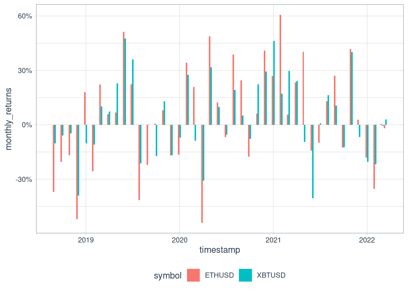
gganimate makes it easy to visualise those exciting (or worrisome, depending which side of the trade you were on…!) periods of high volatility.
A personal favourite was the parabolic rise in late 2017…
vol <- map_bucket_trades(start_date = "2017-08-05",
                         end_date = "2017-12-25",
                         symbol = "XBTUSD",
                         binSize = "1h")


p <- vol %>%
  filter(timestamp <= "2017-12-17") %>%
  ggplot(aes(x = timestamp, y = close)) +
  geom_candlestick(aes(open = open, high = high, low = low, close= close),
                   fill_up = "green",
                   fill_down = "red",
                   colour_up = "green",
                   colour_down = "red") +
  scale_y_continuous(labels = scales::dollar) +
  transition_time(timestamp) +
  shadow_mark() +
  theme_minimal() +
  view_follow()

animate(p, end_pause = 5)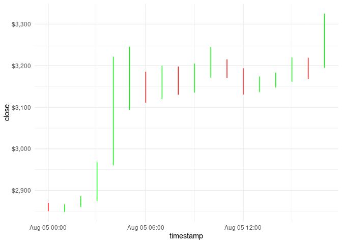
…but I’ll spare the pain of showing what came next…!
References
Dancho, Matt, and Davis Vaughan. 2020. Tidyquant: Tidy Quantitative Financial Analysis. https://CRAN.R-project.org/package=tidyquant.
Pedersen, Thomas Lin, and David Robinson. 2020. Gganimate: A Grammar of Animated Graphics. https://CRAN.R-project.org/package=gganimate.