library(tidyverse)
library(bnlearn)
library(gt)

injuries <- read.csv("injuries.csv") %>%
mutate(across(where(is.character), as.factor))Investigating sports injuries with Bayesian networks using {bnlearn}.
R
Bayesian Network
This post explores the use of Bayesian networks with the excellent {bnlearn} package to examine the relationship between different risk factors and the probability of sustaining a sports injury.
Introduction
In this post I want to share a few details about the humble Bayesian Network (BN). While not generally considered one of the “mainstream” forms of analysis, Bayesian networks have several features that make them an interesting choice, including their flexibility, interpretability and visually appealing nature. I used BNs during PhD, and was fortunate enough to receive some guidance from Marco Scutari, the author of bnlearn, and who is a leading expert in the field when it comes to all things BN. From the outset, I want to clarify that I am by no means an expert in Bayesian networks (far from it!), and encourage any reader who wants to learn more about the theory underlying BNs, or to see more in depth examples, to visit Marco’s site which is a fantastic place to start. I have also included a list of resources I found helpful when learning about BNs at the end of the post. That said, in this post I hope to show a motivating example that might spark some ideas about how BNs can be used!
So what is a Bayesian network?
Wikipedia actually provides a nice overview, so I’ll cheat paraphrase from there…
A Bayesian network is a probabilistic graphical model that represents a set of variables and their conditional dependencies via a directed acyclic graph (DAG). Bayesian networks are ideal for taking an event that occurred and predicting the likelihood that any one of several possible known causes was the contributing factor. For example, a Bayesian network could represent the probabilistic relationships between diseases and symptoms. Given symptoms, the network can be used to compute the probabilities of the presence of various diseases.
So in really simple terms, a Bayesian network allows us to ask questions like “if the value of variable A is x and the value of variable B is y, what is the probability variable C of being value z?” Or, if the weather is looking overcast, and it rained yesterday, what is the probability the it will rain today?
There are some other important features that I am going to bullet point here for brevity:
- Nodes are variables in the networks, arcs are links between nodes.
- Networks can be discrete (all variables are categorical), or continuous or a hybrid of both.
- The structure of a network can be specified ahead of time if it is known, or it can learnt from the data, or a hybrid approach where both “expert knowledge” and a data driven approach to learning can be combined.
- There are a range of different algorithms in
bnlearnthat can be used to learn a structure of a network from the data. - Once a network has been learnt, it can be queried or used for predictions.
For me personally, the visual nature of Bayesian networks is really appealing, something which I’ll hopefully demonstrate in the following examples.
Enough theory, some examples!
The data I’ve used here comes from my PhD, where I was investigating the relationships between stress-related factors and the risk of sports injury. I have simplified the data slightly here just to make the examples clearer. If interested in the full study, you can find the paper in published form here and the git repo for the paper here.
The data contains the following variables:
- injured: Whether an injury was sustained during the study period
- pi: Previous injury, whether the participant had sustained an injury in the 6 months preceding the study
- gender: Gender of the participant
- ind_team: Whether the participant competes in an individual or team sport
- clevel: Competitive level, The highest level the participant had reached in competition
- hours: Number of hours spent training per week
- nlebase: Baseline negative life events
- ri: Reward Interest (personalty characteristic)
- fffs: Fight-Flight-Freeze System (personalty characteristic)
- bis: Behavioural Inhibition System (personalty characteristic)
- stiffness: Sum of all lower body stiffness locations
- balance: Score on a balance test, higher score = poorer balance.
- hrv: Heart rate variability, Root mean squared difference of successive RR intervals.
Data can be found here: https://raw.githubusercontent.com/hfshr/distill_blog/master/_posts/2020-11-01-bayesian-networks-with-bnlearn/injuries.csv
Each variable has two levels, as shown below:
injuries %>%
  gather(var, value) %>%
  count(var, value) %>%
  select(-n) %>%
  mutate(level = ifelse(row_number() %% 2 == 0, "Level 1", "Level 2")) %>%
  pivot_wider(names_from = level, values_from = "value") %>%
  select(Variable = var, "Level 1", "Level 2") %>%
gt()| Variable | Level 1 | Level 2 |
|---|---|---|
| balance | Low | High |
| bis | Low | High |
| clevel | national_international | club_university_county |
| fffs | Low | High |
| gender | male | female |
| hours | Low | High |
| hrv | Low | High |
| ind_team | team | individual |
| injured | injured | healthy |
| nlebase | Low | High |
| pi | no injury | injury |
| ri | Low | High |
| stiffness | Low | High |
Network preparation
To start, I simply extract the names of the variables into two character strings, one for the “explanatory” variables and one for the “control” variables. I’ll use these character vectors in later steps.
# select names of measured variables
explanatory_vars <- injuries %>%
  select(stiffness:fffs, injured) %>%
  names()

# select names of "explanatory" variables, e.g., gender
control_vars <- injuries %>%
  select(pi:hours) %>%
  names()
Next, I create a blacklist to restrict certain arcs between specific nodes from being learnt in the network. Specifically, I restrict the direction of the arcs from control \(\rightarrow\) explanatory and restrict some arcs between the control variables, as these are not of interest.
## create blacklist

black_list <- expand.grid(
  from = explanatory_vars,
  to = control_vars
) %>%
  bind_rows(
    .,
    data.frame(
      from = c("clevel", "nlebase", "nlebase"),
      to = c("gender", "ind_team", "gender")
    )
  )
I also enforce a relationship between nlebase \(\rightarrow\) injured. This is a relationship is often found in the literature, although for reasons I won’t get into here wasn’t apparent in the data I collected, but I still wanted to include this relationship in my analysis.
## create whitelist
white_list <- data.frame(
  from = c("nlebase"),
  to = c("injured")
)
Fitting the network
In bnlearn there are several algorithms available that can be used to learn the structure (for the full list see https://www.bnlearn.com/). In this example, I have chosen the tabu search algorithm - a score-based algorithm that explores the search space starting from a simple network structure and adding, deleting, or reversing one arc at a time until the score can no longer be improved (Olmedilla et al. 2018). I have also used the boot.strength function that allows n networks to be learnt via bootstrap samples. This enables the strength of each arc to be estimated by the number of times that particular arc is learnt during the sampling process.
I’ve only used 100 repeats here for speed, in the real world you might consider using more to ensure robustness.
# set seed for reproducibility
set.seed(122)

str_network <- boot.strength(
  injuries,
  algorithm = "tabu",
  algorithm.args = list(
    blacklist = black_list,
    whitelist = white_list,
    tabu = 100
  )
)
Using the averaged.network function, I select all the arcs that were present in at least 30% of the learnt networks, this is equivalent to an arc strength of 0.3. An arc strength of 1 indicates that the arc was always present in the network, with the value decreasing as arcs were found in fewer networks.
avg30 <- averaged.network(str_network, threshold = 0.30)We can now plot the network to visualise the relationships that have been learnt. I use the strength.plot function which shows the strength of the relationship between arcs via different line styles in the plot. Thin, dashed arcs indicate the weakest arcs (arc strength below 0.50), whereas thick solid arcs indicate the strongest arcs (arc strengths approaching 1).
library(Rgraphviz)

gR <- strength.plot(
  avg30,
  str_network,
  shape = "rectangle",
  render = FALSE,
  groups = list(explanatory_vars, control_vars),
  layout = "dot"
)

# Colour the variables of interest
nodeRenderInfo(gR)$fill[explanatory_vars] <- "deepskyblue"

# Colour the main outcome variable
nodeRenderInfo(gR)$fill["injured"] <- "gold"

# Show me the network!
renderGraph(gR)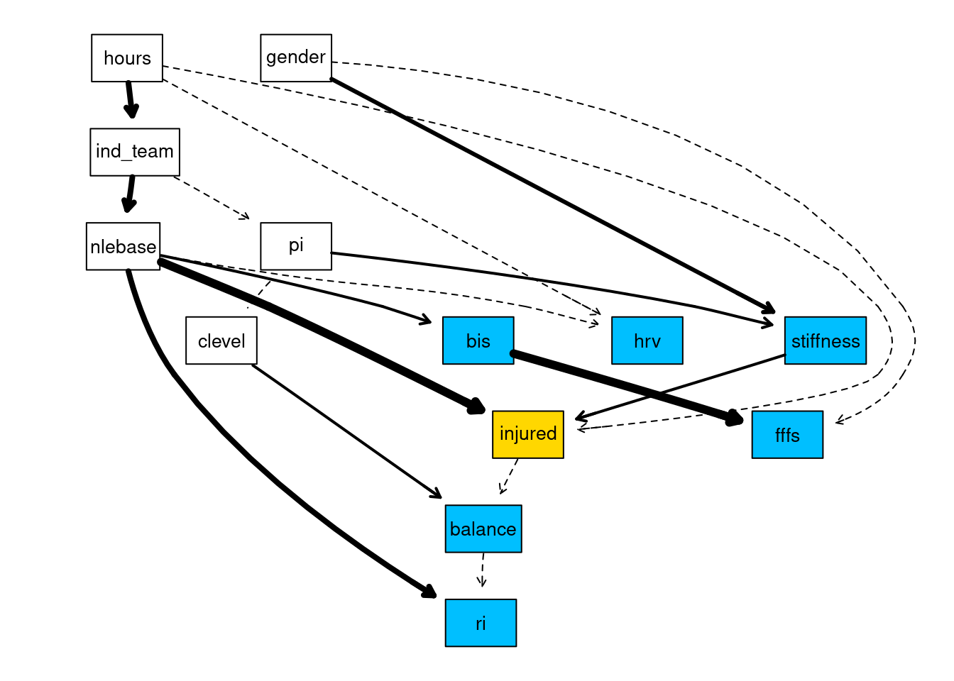
Interrogating the network
Now we have learnt the network structure, we can use the network to answer queries about the probabilistic relationships in the network. This is achieved thorough using the conditional probabilities tables that give us the probability of an event, given other events. For example, take the stiffness node from the network above. We see there are two arcs linked to the stiffness node, pi \(\rightarrow\) stiffness and gender \(\rightarrow\) stiffness. To see these probability tables we can simple use:
# fit the network to the data
fitted <- bn.fit(cextend(avg30), injuries)

# Conditional probabilities for the stiffness node
fitted$stiffness$prob
, , gender = female
pi
stiffness injury no injury
High 0.7333333 0.1304348
Low 0.2666667 0.8695652
, , gender = male
pi
stiffness injury no injury
High 0.6336634 0.6086957
Low 0.3663366 0.3913043We can use this information to make a number of statements, for example, females with a previous injury (pi) are more likely to have “High” stiffness compared to males.
We may want to be a little more specific with our queries, for example say we want to know what the probability of an injury when stiffness == “High”. We can use bnlearn::cpquery() to ask this very question.
I’ve used likelihood weighting here(method = “lw”) which is an approximate inference algorithm based on Monte Carlo simulations, so you may get slightly different results when running this. Use ?bnlearn::cpquery to see the different options available for sampling.
# ask the query
cpquery(fitted,
  event = (injured == "injured"),
  evidence = list(stiffness = "High"),
  method = "lw"
)
[1] 0.302661Likewise we can ask the same question for when stiffness == “Low”
cpquery(fitted,
  event = (injured == "injured"),
  evidence = list(stiffness = "Low"),
  method = "lw"
)
[1] 0.1759626We can see that High stiffness almost doubles the probability of injury.
Now, this can get a little repetitive when you want to investigate lots of variables with different combinations, so I created a function that enables multiple variables to be passed in. It’s a bit lengthy and could probably be simplified a little, but it does the job…!
probability_generator <- function(.data, vars, outcome, state, model, repeats = 500000) {
  all.levels <- if (any(length(vars) > 1)) {
    lapply(.data[, (names(.data) %in% vars)], levels)
  } else {
    all.levels <- .data %>%
      select(all_of(vars)) %>%
      sapply(levels) %>%
      as_tibble()
  }
  combos <- do.call("expand.grid", c(all.levels, list(stringsAsFactors = FALSE))) # al combiations

  # generate character strings for all combinations
  str1 <- ""
  for (i in seq(nrow(combos))) {
    str1[i] <- paste(combos %>% names(), " = '",
      combos[i, ] %>% sapply(as.character), "'",
      sep = "", collapse = ", "
    )
  }

  # repeat the string for more than one outcome
  str1 <- rep(str1, times = length(outcome))
  str1 <- paste("list(", str1, ")", sep = "")

  # repeat loop for outcome variables (can have more than one outcome)
  all.levels.outcome <- if (any(length(outcome) > 1)) {
    lapply(.data[, (names(.data) %in% outcome)], levels)
  } else {
    all.levels <- .data %>%
      select(all_of(outcome)) %>%
      sapply(levels) %>%
      as_tibble()
  }
  combos.outcome <- do.call("expand.grid", c(all.levels.outcome))

  # repeat each outcome for the length of combos
  str3 <- rep(paste("(", outcome, " == '", state, "')", sep = ""), each = length(str1) / length(outcome))

  # fit the model with bayes method
  fitted <- bn.fit(cextend(model), .data, method = "bayes", iss = 1)

  # join all elements of string together
  cmd <- paste("cpquery(fitted, ", str3, ", ", str1, ", method = 'lw', n = ", repeats, ")", sep = "")

  prob <- rep(0, length(str1)) # empty vector for probabilities
  for (i in seq(length(cmd))) {
    prob[i] <- eval(parse(text = cmd[i]))
  } # for each combination of strings, what is the probability of outcome
  res <- cbind(combos, prob)

  return(res)
}
Now, we know that the injured node is of the most interest here, so we might want to know what effect all the nodes that are connected to the injured node have on the probability of being injured. To find out what these other nodes are we can find the “Markov blanket” for the injured node. A Markov blanket contains all the nodes that make the node of interest conditionally independent from the rest of the network (Fuster-Parra et al. 2017), and we can use the bnlearn::mb to find these nodes.
For example for the injured node we can do:
mb(avg30, "injured")[1] "nlebase" "clevel" "hours" "stiffness" "balance" and we find five nodes of interest.
With our probability_generator function, we can now pass in these nodes and find out the probability of the injured node being in the injured state for every combination of the nodes in the markov blanket. Remember each node can contains only two possible states, so we should end up with 2^5 = 32 combinations.
markov_blanket <- mb(avg30, "injured")

res <- probability_generator(injuries,
  vars = markov_blanket,
  outcome = "injured",
  state = "injured",
  model = avg30
)

# Check number of rows, should = 32
nrow(res)
[1] 3232 combinations may be a bit much to look at, so here I make a quick function to get the top 3 highest and lowest probabilities for comparison.
toptail <- function(data, n) {
  data %>%
    top_n(n, prob) %>%
    bind_rows(., data %>%
      top_n(n, -prob))
}

res %>%
  toptail(., 3) %>%
  arrange(desc(prob)) %>%
  select(Probability = prob, everything()) %>%
  gt() %>%
  tab_row_group(
    group = "Low risk",
    rows = Probability <= 0.25
  ) %>%
  tab_row_group(
    group = "High risk",
    rows = Probability > 0.25
  ) %>%
  tab_options(row_group.font.weight = "bold") %>%
  cols_align("center") %>%
fmt_number(columns = "Probability", decimals = 2)| Probability | nlebase | clevel | hours | stiffness | balance |
|---|---|---|---|---|---|
| High risk | |||||
| 0.51 | Low | club_university_county | High | High | High |
| 0.43 | Low | national_international | High | High | Low |
| 0.41 | Low | national_international | High | High | High |
| Low risk | |||||
| 0.05 | Low | national_international | Low | Low | Low |
| 0.05 | Low | national_international | Low | Low | High |
| 0.04 | Low | club_university_county | Low | Low | Low |
So from this we can conclude those athlete who have “High” combination of training hours, muscle stiffness and poor balance (“High” in this case means a worse score on a balance test) have a much higher risk of injury than those athletes with the opposite profile. Coaches or athletes could use this information to try and reduce their risk of injury by improving their balance or lowering their training hours in a run up to competition. The simple interpretations make this a particularly useful tool in applied settings, which I think is really important.
Bonus visulaisation with {bnviewer}
I recently found the bnviewer package which provides an alternative way to visualising networks generated in bnlearn by leveraging the powerful visNetwork package (that uses vis.js under the hood). Below I plot our network using strength.viewer function, and the results are pretty cool!
You can drag the nodes around and hover over them for more information regarding the arcs. Also looks better in dark mode - click the light bulb in the site header!
library(bnviewer)


strength.viewer(
    bayesianNetwork = avg30,
  bayesianNetwork.boot.strength = str_network,
  bayesianNetwork.arc.strength.threshold.expression = c(
    "@threshold > 0 & @threshold < 0.5",
    "@threshold >= 0.5 & @threshold <= 0.8",
    "@threshold > 0.8 & @threshold <= 1"
  ),
    bayesianNetwork.arc.strength.threshold.expression.color  = c(
      "red", "yellow", "blue"),
    bayesianNetwork.arc.strength.label = TRUE,
    bayesianNetwork.arc.strength.label.prefix = "",
    bayesianNetwork.arc.strength.tooltip = TRUE,
    bayesianNetwork.edge.scale.label.min = 14,
    bayesianNetwork.edge.scale.label.max = 14,
    bayesianNetwork.width = "100%",
    bayesianNetwork.height = "800px",
    bayesianNetwork.layout = "layout_with_sugiyama",
    node.colors = list(background = "gray",
                        border = "#2b7ce9",
                        highlight = list(background = "#e91eba",
                                        border = "#2b7ce9")),

    node.font = list(face="Arial"),
    edges.dashes = FALSE
)
Summary
So that was a very quick intro to Bayesian Networks! As promised, below I have included some resources that I’d highly recommend if you want to take a deeper dive into Bayesian networks. Thanks for reading!
Resources
https://www.bnlearn.com/ - Marco’s / bnlearn website
https://kevintshoemaker.github.io/NRES-746/BayesianNetworks-1.html - a great blog post about BNs
https://bookdown.org/robertness/causalml/docs/tutorial-probabilistic-modeling-with-bayesian-networks-and-bnlearn.html another good starting point covering the basics
https://www.frontiersin.org/articles/10.3389/fvets.2020.00073/full Kratzer et al., (2020) paper I found while writing this post that gives a great walkthough, although not using bnlearn.
References
Fuster-Parra, P., J. Vidal-Conti, P. A. Borràs, and P. Palou. 2017. “Bayesian networks to identify statistical dependencies. A case study of Spanish university students’ habits.” Informatics for Health and Social Care 42 (2): 166–79. https://doi.org/10.1080/17538157.2016.1178117.
Olmedilla, Aurelio, Víctor J. Rubio, Pilar Fuster-Parra, Constanza Pujals, and Alexandre García-Mas. 2018. “A Bayesian approach to sport injuries likelihood: Does player’s self-efficacy and environmental factors plays the main role?” Frontiers in Psychology 9: 1–10. https://doi.org/10.3389/fpsyg.2018.01174.